Paper Read 4 - Introduction to Inverse Kinematics with Jacobian Transpose, Pseudoinverse and Damped Least Squares methods
In this post, I am going to document my learning process of Jacobian Transpose, Pseudoinverse and Damped Least Squares methods, which complement post 4. In addition to this, there is the learning of Selectively Damped Least Squares methods.
Introduction
Want the end effectors to track the target positions and to do a reasonable job even when the target positions are in unreachable positions:
-
Difficult to completely eliminate the possibility of unreachable positions;
-
Target positions are barely reachable and can be reached only with full extension of the links, then the situation is very similar to having unreachable targets;
Preliminaries: forward kinematics and Jacobians
\[\mathbf{t}_i=\mathbf{s}_i(\boldsymbol{\theta}), \quad \text { for all } i\] \[\dot{\overrightarrow{\mathbf{s}}}=J(\boldsymbol{\theta}) \dot{\boldsymbol{\theta}}\] \[\boldsymbol{\theta}:=\boldsymbol{\theta}+\Delta \boldsymbol{\theta}\]The change in end effector positions caused by this change in joint angles can be estimated as:
\[\Delta \overrightarrow{\mathbf{s}} \approx J \Delta \boldsymbol{\theta}\]The update of the joint angles can be used in two modes:
-
Each simulation step performs a single update, the end effector positions approximately follow the target positions.
-
The joint angles are updated iteratively until sufficiently close to a solution.
-
Use a hybrid of 1 and 2, using a small number of repeated updates.
The rest of this paper discusses strategies for choosing ∆θ to update the joint angles.
Setting target positions closer. When the target positions are too distant, the multibody’s arms stretch out which is usually near a singularity. One technique is to move the target positions in closer to the end effector positions. Change the definition of \(\overrightarrow{\mathbf{e}}\); instead of merely setting \(\overrightarrow{\mathbf{e}}=\overrightarrow{\mathbf{t}}-\overrightarrow{\mathbf{s}}\), \(\overrightarrow{\mathbf{e}}\) has its length clamped. \(\mathbf{e}_i=\operatorname{ClampMag}\left(\mathbf{t}_i-\mathbf{s}_i, D_{\max }\right),\)
where
\[\operatorname{ClampMag}(\mathbf{w}, d)= \begin{cases}\mathbf{w} & \text { if }\|\mathbf{w}\| \leq d \\ d \frac{\mathbf{w}}{\|\mathbf{w}\|} & \text { otherwise }\end{cases}\]Here \(\|\mathbf{w}\|\) represents the usual Euclidean norm. The value \(D_{\max }\) is an upper bound on how far we attempt to move an end effector in a single update step.
The pseudoinverse method
\[\Delta \boldsymbol{\theta}=J^{\dagger} \overrightarrow{\mathbf{e}}\]The pseudoinverse have stability problems in the neighborhoods of singularities. If the configuration is exactly at a singularity, then the pseudoinverse will be well-behaved. If the configuration is close to a singularity, then the pseudoinverse method will lead to very large changes in joint angles for small movements in the target position.
The pseudoinverse has the further property that the matrix \(\left(I-J^{\dagger} J\right)\) performs a projection onto the nullspace of \(J\). Therefore, for all vectors \(\varphi\), \(J\left(I-J^{\dagger} J\right) \boldsymbol{\varphi}=\mathbf{0}\).
\[\Delta \boldsymbol{\theta}=J^{\dagger} \overrightarrow{\mathbf{e}}+\left(I-J^{\dagger} J\right) \varphi\]for any vector \(\varphi\) and still obtain a value for \(\Delta \boldsymbol{\theta}\) which minimizes the value \(J \Delta \boldsymbol{\theta}-\overrightarrow{\mathbf{e}}\). By suitably choosing \(\varphi\), one can try to achieve secondary goals in addition to having the end effectors track the target positions.
Damped least squares
Rather than just finding the minimum vector \(\Delta \boldsymbol{\theta}\) that gives a best solution to \(\overrightarrow{\mathbf{e}}=J \Delta \boldsymbol{\theta}\), we find the value of \(\Delta \boldsymbol{\theta}\) that minimizes the quantity \(\|J \Delta \boldsymbol{\theta}-\overrightarrow{\mathbf{e}}\|^2+\lambda^2\|\Delta \boldsymbol{\theta}\|^2\).
Then
\[\Delta \boldsymbol{\theta}=J^T\left(J J^T+\lambda^2 I\right)^{-1} \overrightarrow{\mathbf{e}} .\]The damping constant should large enough so that the solutions for \(\Delta \boldsymbol{\theta}\) are well-behaved near singularities, but if it is chosen too large, the convergence rate is too slow.
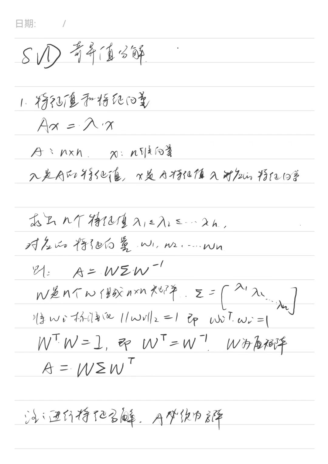
Singular value decomposition
The singular value decomposition (SVD) provides a powerful method for analyzing the pseudoinverse and the damped least squares methods.
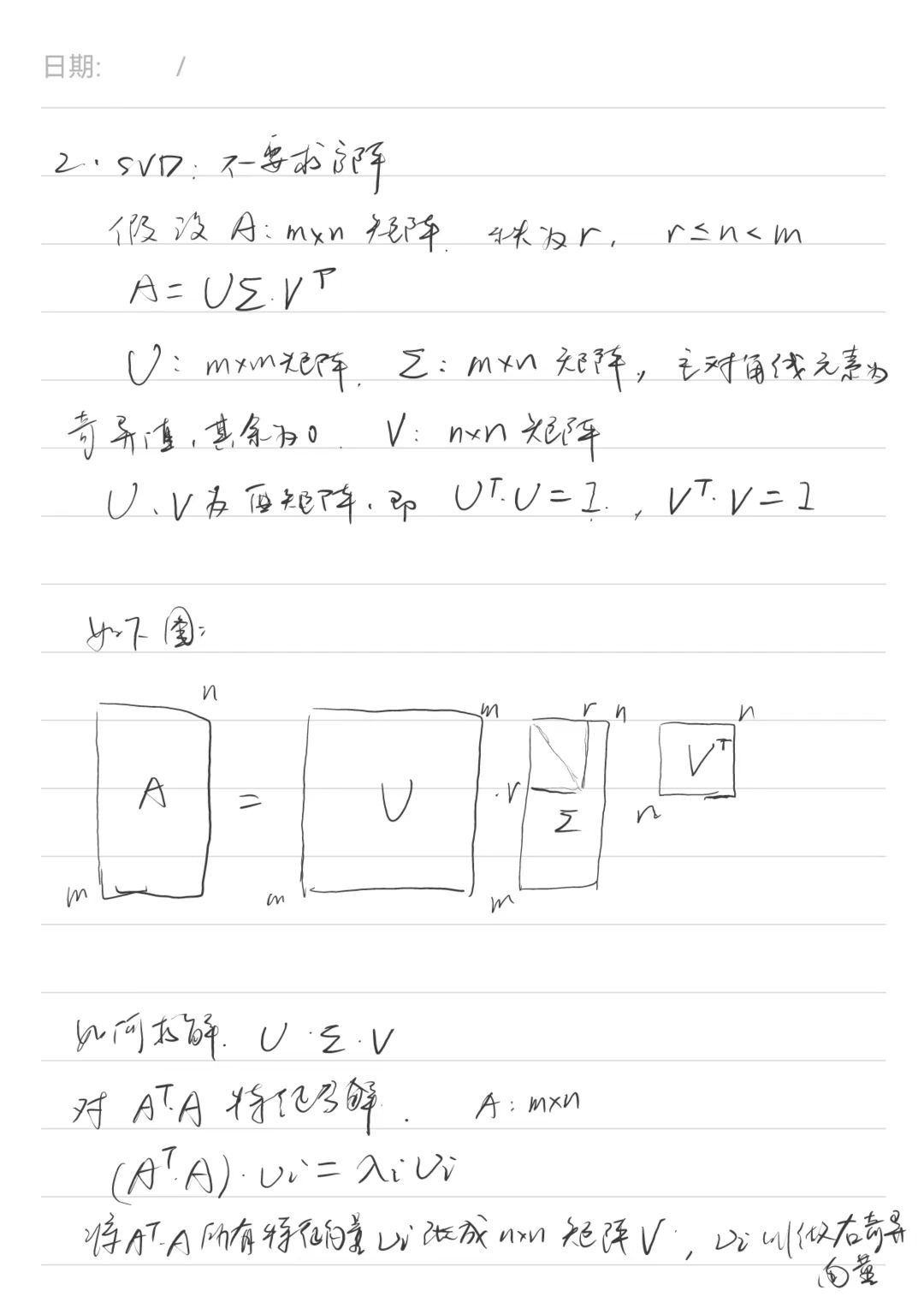
\[J=U D V^T,\]where \(U\) and \(V\) are orthogonal matrices and \(D\) is diagonal. If \(J\) is \(m \times n\), then \(U\) is \(m \times m\), \(D\) is \(m \times n\), and \(V\) is \(n \times n\).
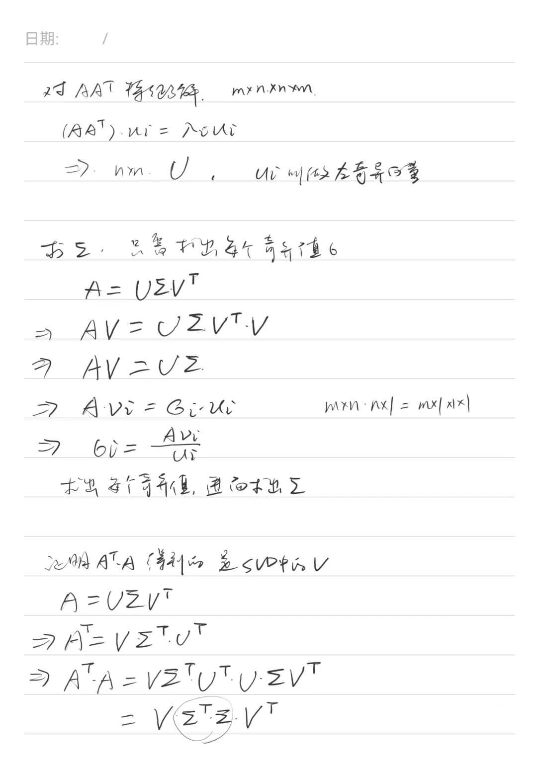
Use \(\mathbf{u}_i\) and \(\mathbf{v}_i\) to denote the i th columns. The orthogonality of \(U\) and \(V\) implies that the columns form an orthonormal basis for \(\mathbb{R}^m\) (\(\mathbb{R}^n\) ). The vectors \(\mathbf{v}_{r+1}, \ldots, \mathbf{v}_n\) are an orthonormal basis for the nullspace of \(J\). \(J\) can be written in the form
\[J=\sum_{i=1}^m \sigma_i \mathbf{u}_i \mathbf{v}_i^T=\sum_{i=1}^r \sigma_i \mathbf{u}_i \mathbf{v}_i^T .\]The transpose, \(D^T\), of \(D\) is the \(n \times m\) diagonal matrix with diagonal entries \(\sigma_i=d_{i, i}\). The product \(D D^T\) is the \(m \times m\) matrix with diagonal entries \(d_{i, i}^2\). The pseudoinverse, \(D^{\dagger}=\left(d_{i, j}^{\dagger}\right)\) is the \(n \times m\) diagonal matrix with diagonal entries
\[d_{i, i}^{\dagger}= \begin{cases}1 / d_{i, i} & \text { if } d_{i, i} \neq 0 \\ 0 & \text { if } d_{i, i}=0 .\end{cases}\]The pseudoinverse of \(J\) is equal to
\[J^{\dagger}=V D^{\dagger} U^T .\]Thus,
\[J^{\dagger}=\sum_{i=1}^r \sigma_i^{-1} \mathbf{v}_i \mathbf{u}_i^T .\]The damped least squares method is also easy to understand with the SVD.
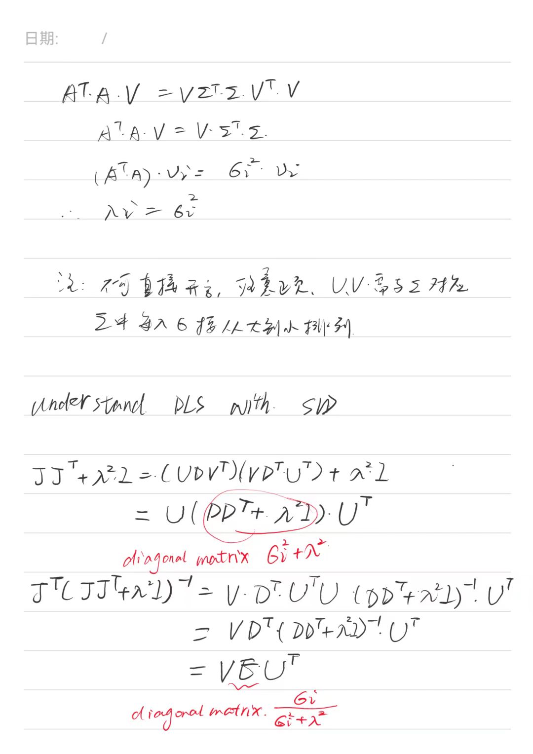
\[J J^T+\lambda^2 I=\left(U D V^T\right)\left(V D^T U^T\right)+\lambda^2 I=U\left(D D^T+\lambda^2 I\right) U^T .\]The matrix \(D D^T+\lambda^2 I\) is the diagonal matrix with diagonal entries \(\sigma_i^2+\lambda^2\) and its inverse is the \(m \times m\) diagonal matrix with non-zero entries \(\left(\sigma_i^2+\lambda^2\right)^{-1}\). Then,
\[J^T\left(J J^T+\lambda^2 I\right)^{-1}=V D^T\left(D D^T+\lambda^2 I\right)^{-1} U^T=V E U^T\]where \(E\) is the \(n \times m\) diagonal matrix with diagonal entries equal to
\[e_{i, i}=\frac{\sigma_i}{\sigma_i^2+\lambda^2}\]Thus, the damped least squares solution
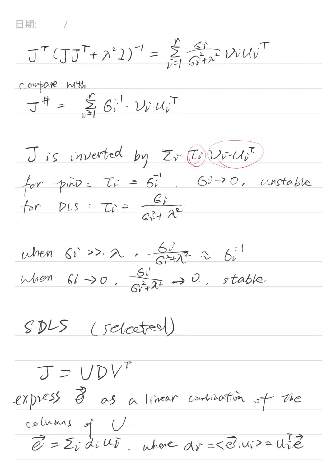
\[J^T\left(J J^T+\lambda^2 I\right)^{-1}=\sum_{i=1}^r \frac{\sigma_i}{\sigma_i^2+\lambda^2} \mathbf{v}_i \mathbf{u}_i^T\]Compare with
\[J^{\dagger}=\sum_{i=1}^r \sigma_i^{-1} \mathbf{v}_i \mathbf{u}_i^T .\]In both cases, \(J\) is “inverted” by an expression \(\sum_i \tau_i \mathbf{v}_i \mathbf{u}_i^T\). For pseudoinverses, the value \(\tau_i\) is just \(\sigma_i^{-1}\) (setting \(0^{-1}=0\) ); for damped least squares, \(\tau_i=\sigma_i /\left(\sigma_i^2+\lambda^2\right)\). The pseudoinverse method is unstable as \(\sigma_i\) approaches zero; in fact, it is exactly at singularities that \(\sigma_i\) ‘s are equal to zero.
The damped least squares method tends to act similarly to the pseudoinverse method away from singularities and effectively smooths out the performance of pseudoinverse method in the neighborhood of singularities.
Derivation of relevant formula
Experimental results
- The Jacobian transpose performed poorly in multiple end effectors, but works well in single end effector. For these applications, the Jacobian transpose is fast and easy to implement.
- The pseudoinverse method worked very poorly whenever the target positions were out of reach.
- The damped least squares method worked better than the Jacobian transpose method in multiple end effectors, although slower. Set the damping constant λ to minimize the average error of the end effectors’s positions, but cause oscillation and shaking.
- A good idea to clamp the maximum angle change in a single update to avoid bad behavior from unwanted large instantaneous changes in angles.