Cable Driven Manipulator 2 - Kinematics
The kinematics consists of two layers of models, firstly for the transformation relation from joint space to Cartesian space for the overall kinematic properties of the manipulator, and additionally to analyse the transformation relation from drive space to joint space.
Joint space to Cartesian space
Latest kinematics code implementation is in my repository cable_driven_manipulator, including forward kinematics, inverse kinematics, Jacobian matrices, etc.
Version 2.1
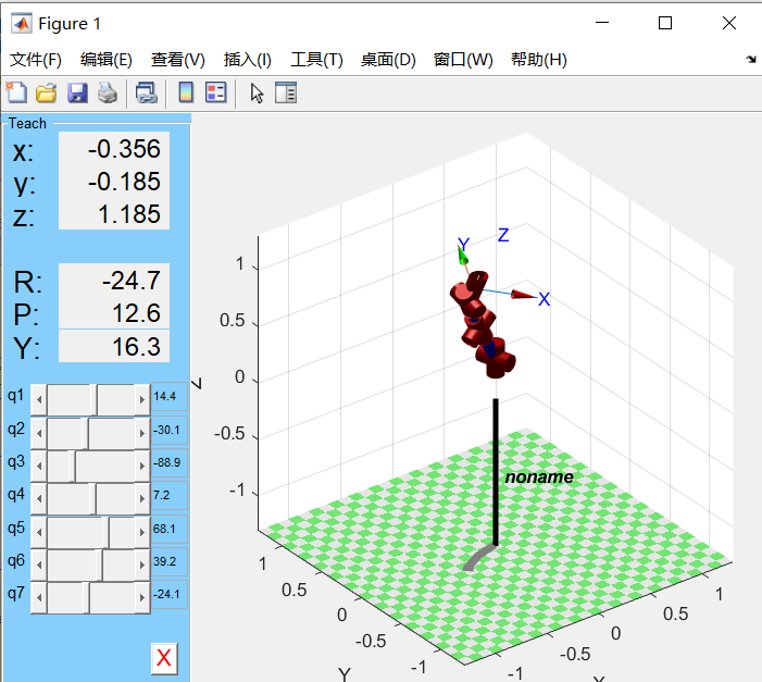
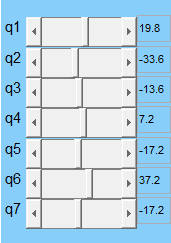
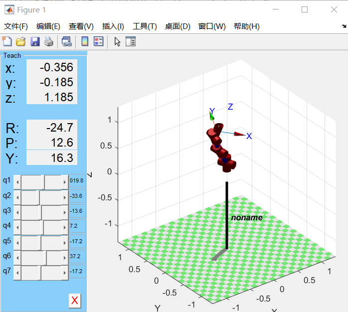
Supplement KUKA LBR iiwa manipulator demo, completing inverse kinematics based on gradient projection method (GPM).
Assume \(\theta5\) has max as pi/2 and min as pi/3.
 |
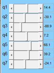 |
Figure 1 Target Angle | Figure 2 Result Angle |
We can see that \(\theta5\) is limited.
Version 2.0
Based on the purpose of effect visualisation, function encapsulation other than inverse kinematics is completed.
Add KUKA LBR iiwa manipulator demo, completing inverse kinematics based on Damped Least Square (DLS) method.
 |
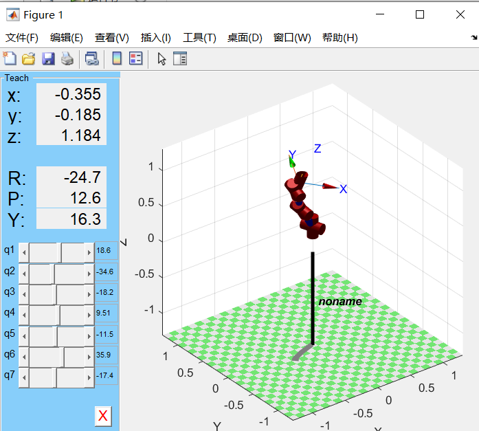 |
Figure 1 Target 6D Pose | Figure 2 Result 6D Pose |
Version 1.0
Algorithm validation using PUMA560 as an example:
close all,
clear,clc;
%% Modified DH parameters
L1 = Link([ 0, 0, 0, 0, 0], 'modified');
L2 = Link([ 0, 0, -0.03, -pi/2, 0], 'modified');
L3 = Link([ 0, 0, 0.34, 0, 0], 'modified');
L4 = Link([ 0, 0.338, -0.04, -pi/2, 0], 'modified');
L5 = Link([ 0, 0, 0, pi/2, 0], 'modified');
L6 = Link([ 0, 0, 0, -pi/2, 0], 'modified');
robot_modified = SerialLink([L1,L2,L3,L4,L5,L6]);
% robot_modified.display();
robot_modified.teach([0 0 0 0 0 0]);
theta_target = [deg2rad(10.8), deg2rad(-3.6), deg2rad(-3.6), deg2rad(7.2), deg2rad(-7.2), deg2rad(7.2)];
p_target = robot_modified.fkine(theta_target);
q = rad2deg(robot_modified.ikine(p_target));
%% 正运动学手搓好使
% alpha = [0 -pi/2 0 -pi/2 pi/2 -pi/2];
% d = [0 0 0 0.338 0 0];
% a = [0 -0.03 0.34 -0.04 0 0];
% T06 = eye(4);
% for k = 1:6
% T_XY_1 = cos(theta(k));
% T_XY_2 = -sin(theta(k));
% T_XY_3 = 0;
% T_XY_4 = a(k);
% T_XY_5 = sin(theta(k)) * cos(alpha(k));
% T_XY_6 = cos(theta(k)) * cos(alpha(k));
% T_XY_7 = -sin(alpha(k));
% T_XY_8 = -sin(alpha(k)) * d(k);
% T_XY_9 = sin(theta(k)) * sin(alpha(k));
% T_XY_10 = cos(theta(k)) * sin(alpha(k));
% T_XY_11 = cos(alpha(k));
% T_XY_12 = cos(alpha(k)) * d(k);
%
% T_XY = [T_XY_1 T_XY_2 T_XY_3 T_XY_4;
% T_XY_5 T_XY_6 T_XY_7 T_XY_8;
% T_XY_9 T_XY_10 T_XY_11 T_XY_12;
% 0 0 0 1];
%
% T06 = T06 * T_XY;
% end
%% 逆运动学中雅可比矩阵求解较为复杂,暂时调用Robotics Toolbox
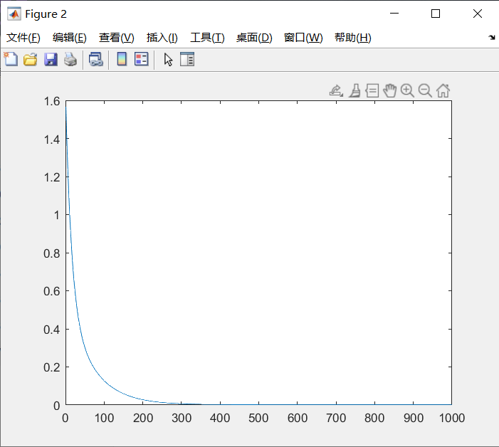
N = 1000;
x_target = p_target.t';
x_ = zeros(1,3);
e = zeros(1,6);
eplot = zeros(1,N);
theta = [0, 0, 0, 0, 0, 0];
for j = 1 : N
%平移
p = robot_modified.fkine(theta);
x_(1:3) = p.t';
e(1:3) = x_target - x_;
%旋转
Rq = t2r(p);
rrr = t2r(p_target) * Rq';
[thn,V] = tr2angvec(t2r(p_target) * Rq');
e(4:6) = thn * V;
eplot(j) = e * e';
Jaco = jacob0(robot_modified, theta);
dq = Jaco' * e';
dq = 0.1 * dq;
theta = theta + dq';
end
thetadeg = rad2deg(theta);
%%
figure();
plot(eplot)
Error design:
e(1:3) is the translation error, which can be calculated from $x_{target} - x$.
e(4:6) is the rotation error, described by the rotation matrix.
Suppose there is a vector called $A_1$ in coordinate system 1, $A_2$ in coordinate system 2, then:
\[A_2=C_1^2A_1\]For the same reason:
\[A_3=C_2^3 A_2\]Then
\[A_3=C_2^3 C_1^2 A_1\]So
\[C_1^3=C_2^3 C_1^2\]This formula describes the conversion of two rotations added together into one larger rotation. That is, the addition of rotations.
So
\[C_2^{3^{-1}} C_1^3=C_1^2\]This would indicate that a large rotation minus a small rotation equals another rotation. That is, subtraction between rotations.
In matrix operation, “inverse” is not easy to find, the best matrix to find is “transpose”. But since the rotated matrix is “orthogonal matrix”, its “transpose” = “inverse”, so not only the error of the rotated matrix must be a rotated matrix, but also the calculation process becomes very simple.
\[C_2^{3^{T}} C_1^3=C_1^2\]References
[1] Peter Corke, MATLAB Robotics Toolbox http://petercorke.com.
[2] SJTU-RoboMaster-Team, Matrix_and_Robotics_on_STM32
[3] J.J.Craig, Introduction to robotics mechanics and control
[4] Buss, S. R. (2004). Introduction to inverse kinematics with Jacobian transpose, pseudoinverse and damped least squares methods. IEEE Journal of Robotics & Automation, 17(1).
[5] Chiaverini, S., Oriolo, G., & Maciejewski, A. A. (2016). Redundant Robots. Cham, Switzerland: Springer.
[6] Woliński, Ł., & Wojtyra, M. (2022). A Novel QP-Based Kinematic Redundancy Resolution Method With Joint Constraints Satisfaction. IEEE Access, 10, 41023-41037. doi: 10.1109/ACCESS.2022.3167403.