Paper Read 3 - Inverse Kinematics
A fundamental problem in robotics - because for any manipulator, the amount you want to control is in the manipulation space, while the amount you can control is in the joint space.
Introduction
In the case of a six-degree-of-freedom manipulator, we represent the position and orientation of the end effector by a Transformation Matrix containing the joint positions, which contains the end effector position w.r.t {0} (a 3×1 vector), and the end effector’s rotation matrix w.r.t {0} (a 3×3 matrix), a total of 12 unknowns, and how can the inverse kinematics be solved at this point?
If it is a 7-DOF manipulator, we say that there are redundant degrees of freedom in the manipulator, and the joints can still move when the end effector is fixed, so how do we find the inverse kinematics?
Analytical Solution is not universal and we will not go into details. Pieper principle, see 台大机器人学之运动学——林沛群
Optimization-based Solution, is the transformation of a problem into an optimisation problem for numerical solution. In mathematical language, this means that the problem is solved by taking the
\[q=f^{-1}(x)\]translates into the problem “Find the joint position q that minimises the difference between the actual end effector position x and the positive kinematically calculated end effector position f(q)”:
\[\min _q e, \text { where } e=(x-f(q))^2\]How to solve the above equation (e.g. using Gradient Descent) is a mathematical problem.
Iterative Method - Jacobian Inverse, which “differentiates” the problem and infinitely approximates it using the inverse of instantaneous kinematics.
\[\dot{x}=J \dot{q} \quad \dot{q}=J^{-1} \dot{x}\]Jacobian Transpose), which is the replacement of the difficult inverse operation with a transpose of the Jacobian matrix from the following equation
\[\tau=J^T F\]Since in the inverse kinematics solution we are not concerned with the dynamics of the system, the above equation can also be written as
\[\dot{q}=J^T \dot{x}\]Jacobian Inverse
Take the example of a 2-DOF manipulator:
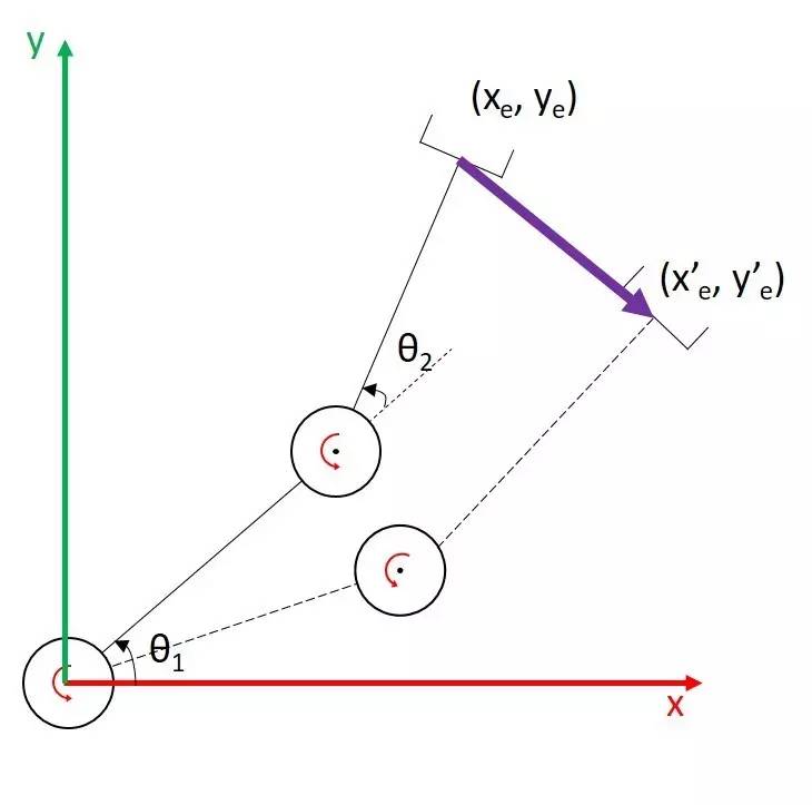
Now we need the end effector to move from (xe, ye) in the diagram along the purple line to (x’e, y’e), but you need to control the joint positions to achieve this. Now there are a couple of ways you can think about this-
Firstly, find only the joint positions corresponding to the start and end points, and directly linearly interpolate these two joint positions to find the joint motion trajectory - this saves a lot of computation, but the end effector is unlikely to follow a straight line;
Second, insert this straight line into many, many intermediate points, each point to find the corresponding joint position, and then control each joint according to this series of joint positions (that is, the analytical/optimisation solution we mentioned earlier);
Thirdly, the line is still inserted into many, many intermediate points, but if the interval between points is small enough and the movement time is short enough, we can invert the Jacobian matrix at each point to find the current change in joint position - in other words, we can also set the speed of movement of the end effector along this line, and use the Jacobian matrix inverse to find the joint velocity, directly controlling the speed of the joint’s motion instead of its position.
We draw the third method as a control block diagram:
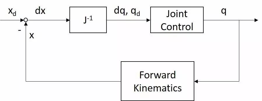
In the diagram xd has a subscript d for “desired”, i.e. the position and orientation you want x to be in, and later on there is a subscript c for “current”, i.e. the current position/orientation of x; we’ll be seeing subscripts like this all the time.
You may not understand the control block diagram, it doesn’t matter, first of all the above line before the Joint control, from left to right it says:
\[\begin{gathered} d x=x_d-x \\ d q=J^{-1} d x \\ q_d=d q+q_c \end{gathered}\]Joint control is where you take your calculated qd and send it to each joint’s controller (e.g. the simplest servo); these controllers ultimately control the joints to position q (with good controllers, q and qd should be very close in most cases).
The bottom line of this diagram says that we have again used positive kinematics from this joint position q to find the end effector position x at this point, which is fed back to the front and given the first equation above to find dx.
Usually you set an xd and the controller needs to go through this control loop a few times to get the dx down to close to 0 (so that x approaches xd), hence this method is also known as the iterative method.
Pseudo-Inverse
What to do when the Jacobian matrix is not invertible? We will discuss one of them here first: the case when the Jacobian matrix is stubby and the robot manipulator has redundant degrees of freedom.
This time to use a mathematical concept called pseudoinverse matrix. There are many kinds of pseudoinverse matrices, and the one that is used more often in robot inverse kinematics is the right pseudoinverse matrix (right-inverse). If the pseudoinverse matrix is denoted as A+, left-inverse means that (A+)A = I; whereas right-inverse means that A(A+) = I.
Right-inverse is obtained by solving the following problem:
\[\begin{gathered} \min _{\dot{q}}\|\dot{q}\|^2 \\ \text { subject to } \dot{x}=J \dot{q} \end{gathered}\]In robotics, we would like to have as little joint motion as possible at each iteration (the least amount of motion out of a number of possible ways of moving), Each move towards the desired goal combines all the joints requiring the least change, i.e. requiring the shortest path in angular space. So what we’re talking about above is finding the smallest possible dq that will satisfy the equation.
Using Lagrange Multiplier, this problem can be turned into:
\[\min _{\dot{q}} \frac{1}{2}\|\dot{q}\|^2+\lambda^T(\dot{x}-J \dot{q})\]The Lagrange multiplier method is the derivative of dq and lamda respectively, and the extreme values are obtained when the derivative is 0:
\[\begin{gathered} \frac{d \frac{1}{2}\|\dot{q}\|^2+\lambda^T(\dot{x}-J \dot{q})}{d \dot{q}}=\dot{q}^T-\lambda^T J=0 \\ \frac{d \frac{1}{2}\|\dot{q}\|^2+\lambda^T(\dot{x}-J \dot{q})}{d \lambda}=\dot{x}-J \dot{q}=0 \end{gathered}\]i.e.
\[\begin{gathered} \dot{q}=J^T \lambda \\ \dot{x}=J \dot{q}=J J^T \lambda \stackrel{\text { solve } \lambda}{\Longrightarrow} \lambda=\left(J J^T\right)^{-1} \dot{x} \\ \dot{q}=J^T\left(J J^T\right)^{-1} \dot{x} \\ \therefore J^{+}=J^T\left(J J^T\right)^{-1} \end{gathered}\]It can be verified that J(J+) = I. The dq solved with this J+ is the minimum joint motion velocity that satisfies the condition.
Finally a brief mention of null space allows us to verify:
\[\forall \dot{q}_0, J\left(I-J^{+} J\right) \dot{q}_0=0\]This means that the matrix I-J(+J) can project any joint velocity into the “null space”, and the projected joint velocity will not cause any motion of the end effector. Using this property, we can use the null space to achieve other tasks (e.g. obstacle avoidance) after the xd of the end effector is satisfied.
Resolved Motion Rate Control of Manipulators and Human Prostheses
Abstract
-
The purpose of deriving resolved motion rate control
-
solutions to problems of coordination, motion under task constraints and appreciation of forces encountered by the controlled hand
Method
\[\frac{d x}{d t}=\dot{x}=J(\theta) \dot{\theta}\]If m > n, J`1 is not defined. If we do not wish to freeze arbitrary coordinates in 6 or add some “elbow” coordinates to x, we may get around the difficulty by defining an optimality criterion, which the manipulator must satisfy while undergoing its motions. For example, minimize
\[G=\frac{1}{2} \int \dot{\boldsymbol{\theta}}^T A \dot{\boldsymbol{\theta}} d t\]A is a positive definite weighting matrix. A simpler criterion is
\[G=\frac{1}{2} \dot{\boldsymbol{\theta}}^T A \dot{\boldsymbol{\theta}}\]That is, the assumed “cost” of motion is approximately the instantaneous weighted system kinetic energy.
With Lagrange multipliers and assuming the desired x_dot is known, we obtain for the optimal theta_dot
\[\dot{\boldsymbol{\theta}}^T=\dot{x}^T\left[J(\boldsymbol{\theta}) A^{-1} J(\boldsymbol{\theta})^T\right]^{-1} J(\boldsymbol{\theta}) A^{-1}\]The above derivation makes plain the influence of A. We may choose A so as to emphasize the role of some components of x and deemphasize others, for example, by heavily penalizing motions of the latter relative to the former.
To synthesize the required A for this purpose, we begin with the cost criterion:
\[G^{\prime}=\frac{1}{2} \dot{x}^T B \dot{x}\]B can usually be chosen by inspection to be positive definite and provide the desired relative emphases. For example, change hand orientation while keeping its location relatively fixed.
\[G^{\prime}=\frac{1}{2} \dot{\boldsymbol{\theta}}^T J^T(\boldsymbol{\theta}) B J(\boldsymbol{\theta}) \dot{\boldsymbol{\theta}}\]Comparing G’ with G, we may identify
\[A=J^T(\boldsymbol{\theta}) B J(\boldsymbol{\theta})\]Note that this A is not necessarily positive definite. What is important, however, is that B be positive definite, and that the resulting A be nonsingular.
DLS (Damped Least Square)
Problems with the Jacobian matrix inverse method
In principle, one of the most obvious requirements for using this method is the dx cannot be too large. Because the Jacobian is constantly changing as the joint positions change, the Jacobian Inverse will no longer be accurate once the joint positions change significantly. This problem can usually be avoided by linear interpolation of the trajectory or by limiting the size of the dx (clamping).
The second difficulty with this method is the Jacobian matrix inverse. Matrix inverse is a very computationally intensive operation. Of course, there are always various ways of solving linear equations to avoid inversions, such as LU decomposition, Chelosky decomposition, QR decomposition, SVD (Singular Value Decomposition).
The biggest problem with this method is still that it doesn’t deal well with robot Singularity or near-Singularity. From the linear equation point of view, when the robot is close to Singularity, the Jacobian matrix becomes more and more ill-conditioned, a small dx may result in a very large dq, and the equations become more sensitive to numerical errors; when the robot is in Singularity, the linear equations may not be solved. When the robot is in Singularity, the linear equations may have no solution, or they may have an infinite number of solutions.
In order to avoid very large joint velocities due to the proximity to Singularity when controlling the manipulator using Jacobi matrix inversion, a natural idea is to limit the joint velocities during the solution process - both to satisfy the equations as much as possible, and also to keep the joint velocities from being too large as much as possible.
For the former, we can solve the equations using the least square method, when the problem can be formulated like this:
\[\min _{\dot{q}}\|J \dot{q}-\dot{x}\|^2\]That is, find a dq that minimises the square of the norm of Jdq - dx; ideally the equations are equal, and the norm is zero.
In the latter case, we want norm of dq to be as small as possible (but obviously not normally 0), so we can add a “damping” term to the above equation to make it look like this:
\[\min _{\dot{q}}\|J \dot{q}-\dot{x}\|^2+\lambda^2\|\dot{q}\|^2\]That is, find a dq such that the sum of the square of the norm of Jdq-dx, plus the square of the norm of dq multiplied by a factor, is minimised. At this point, the size of λ determines which condition “value” more: if λ is very large, then you may get a very small joint velocity, but this velocity will not allow the end effector to follow the trajectory you want; if λ is very small, close to 0, then this method is not much different from the most basic Jacobian Inverse algorithm before. In practice, the size of λ often needs to be chosen carefully.
Solving for the minimum of the above equation:
\[\begin{gathered} \frac{d\|J \dot{q}-\dot{x}\|^2+\lambda^2\|\dot{q}\|}{d \dot{q}}=\frac{d(J \dot{q}-\dot{x})^T(J \dot{q}-\dot{x})+\lambda^2 \dot{q}^T \dot{q}}{d \dot{q}} \\ =\frac{d \dot{q}^T J^T J \dot{q}-\dot{x}^T J \dot{q}-\dot{q}^T J^T \dot{x}+\dot{x}^T \dot{x}+\lambda^2 \dot{q}^T \dot{q}}{d \dot{q}} \\ =2 J^T J \dot{q}-2 J^T \dot{x}+2 \lambda^2 I \dot{q}=0 \end{gathered}\]So we get an equivalent equation:
\[\left(J^T J+\lambda^2 I\right) \dot{q}=J^T \dot{x}\]The coefficient matrix on the left is invertible:
\[\dot{q}=\left(J^T J+\lambda^2 I\right)^{-1} J^T \dot{x}\]i.e.
\[\dot{q}=\left(J^T J+\lambda^2 I\right)^{-1} J^T \dot{x}=J^T\left(J J^T+\lambda^2 I\right)^{-1} \dot{x}\]Because the left side requires the inverse of the matrix size of n × n, n is the number of joints, to be as big as how big; the right side requires the inverse of the matrix size of m × m, m is the size of the degrees of freedom of the operation space, the maximum is certainly not more than six. This small conversion limits the size of the matrix to be inverted and improves the overall speed of the operation.