Paper Read 2 - Instantaneous Kinematics and Jacobian Matrix
Instantaneous kinematics also describes the mapping from joint space to operation space. However, the term “instantaneous” indicates that it does not describe “static” positions, but rather “dynamic” velocities. The function of forward kinematics is shown as follows: \(\begin{aligned} \vec{x} = f(\vec{q}) \end{aligned}\)
q vector represents the joint position and x vector represents the position and orientation of the end effector.
Instantaneous Kinematics
When “instantaneous kinematics” solves for the mapping of velocities from joint space to operation space, since velocity describes a change in position over a short period of time, the derivative of position with respect to time, I’m sure it’s natural for you to think that we need to solve for such a function:
\[\frac{d \vec{x}}{d t}=g\left(\frac{d \vec{q}}{d t}\right)\]or:
\[\dot{x}=g(\dot{q})\]Our task now is to derive the “instantaneous kinematics” formula from the “forward kinematics” formula:
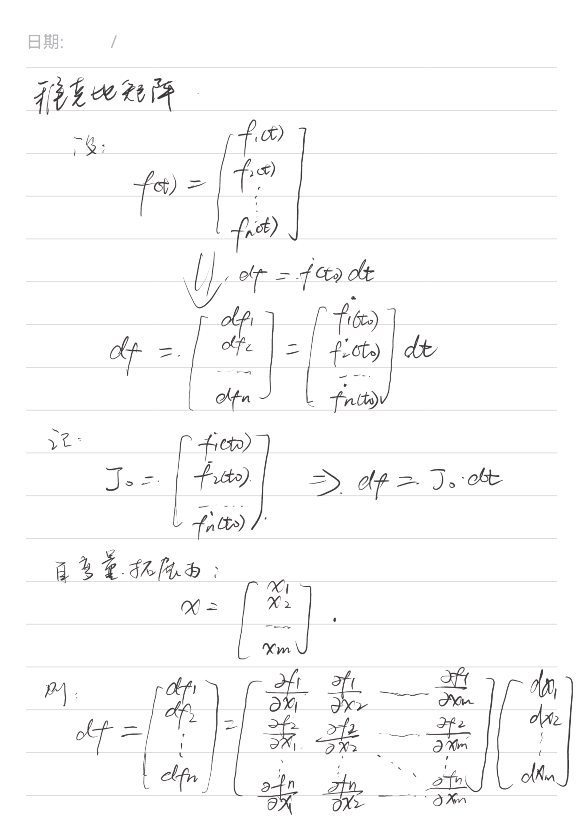
\[\frac{d \vec{x}}{d t}=\frac{d f(\vec{q})}{d t}=\frac{d f(\vec{q})}{d \vec{q}} \cdot \frac{d \vec{q}}{d t}\]i.e. :
\[\dot{x}=\frac{d \vec{x}}{d \vec{q}} \cdot \dot{q}\]What connects the velocities in joint space to the velocities in operation space is the Jacobian matrix obtained from the derivation of the vectors. Now, let’s express this important conclusion mathematically by denoting the derivative of the vector x with respect to the vector q by J:
\[\dot{x}=J \dot{q}\]According to the vector derivation method described at the beginning, J is a matrix. This matrix is not really abstract at all: if we look carefully at each of its elements, we see that its ith row and jth column represent the physical meaning of how the ith translation/rotation direction of the operation space will move when the jth joint moves:
\[J=\left[\begin{array}{ccc} \frac{d x_1}{d q_1} & \cdots & \frac{d x_1}{d q_n} \\ \vdots & \ddots & \vdots \\ \frac{d x_m}{d q_1} & \cdots & \frac{d x_m}{d q_n} \end{array}\right]\]For example, the first row and first column indicate that when the first joint moves a certain angle/distance, the end effector correspondingly moves/rotates a certain distance/angle in the direction of x1. If you still think it’s too abstract, let’s look at an example.
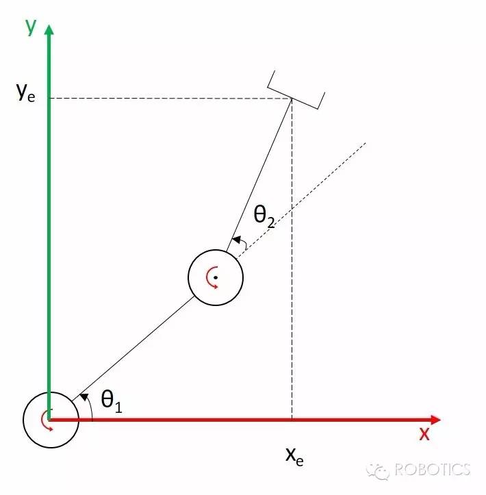
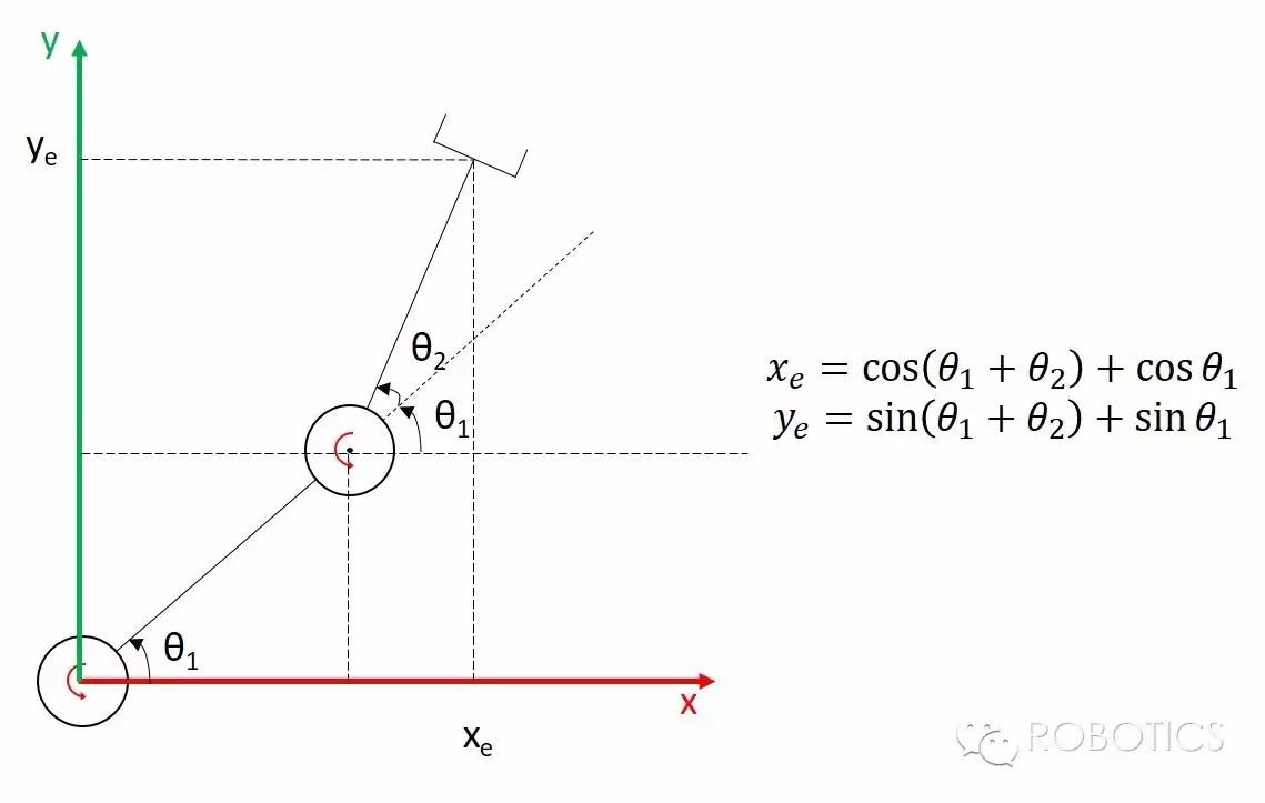
Our joint space is (θ1, θ2) and the operation space is (xe, ye), and we have also written out the forward kinematics formulae (making the lengths of the links all 1):
\[\begin{gathered} x_e=\cos \left(\theta_1+\theta_2\right)+\cos \theta_1 \\ y_e=\sin \left(\theta_1+\theta_2\right)+\sin \theta_1 \end{gathered}\]Then the Jacobian matrix is:
\[J=\left[\begin{array}{ll} \frac{d x_e}{d \theta_1} & \frac{d x_e}{d \theta_2} \\ \frac{d y_e}{d \theta_1} & \frac{d y_e}{d \theta_2} \end{array}\right]=\left[\begin{array}{cc} -\sin \left(\theta_1+\theta_2\right)-\sin \theta_1 & -\sin \left(\theta_1+\theta_2\right) \\ \cos \left(\theta_1+\theta_2\right)+\cos \theta_1 & \cos \left(\theta_1+\theta_2\right) \end{array}\right]\]Note that in our example, there are two degrees of freedom in joint space and two degrees of freedom in operation space, so our Jacobian matrix is square (square matrix); but a Jacobian matrix is not necessarily square.
Consider the substitution when θ1 = 0 and θ2 = 90°, and we get this Jacobian matrix:
\[J=\left[\begin{array}{ll} \frac{d x_e}{d \theta_1} & \frac{d x_e}{d \theta_2} \\ \frac{d y_e}{d \theta_1} & \frac{d y_e}{d \theta_2} \end{array}\right]=\left[\begin{array}{cc} -1 & -1 \\ 1 & 0 \end{array}\right]\]Corresponding to:
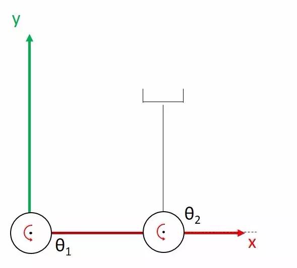
If we keep the first joint motionless and rotate the second joint, then at this one instant the end effector will move only in the x-direction with a velocity of 1 (linear velocity equals the angular velocity multiplied by the radius, i.e. the length of the LINK), and in the y-direction with a velocity of 0, so the second column of the J matrix is [-1, 0].
And if we keep the second joint still and rotate the first joint, the instantaneous velocity of the end effector will be perpendicular to the line connecting the end effector to the axis of the first joint, which has a radius of √2, and the linear velocity will be √2, which breaks down to -1 in the x-direction and 1 in the y-direction, so the first column of the J-matrix is [-1, 1].
\[\dot{x}=J \dot{q}\]This equation shows that the relationship between the velocity of the end effector and the joint velocity is linear! The form of this equation is also exactly the same as the linear equation Ax = b, which we have used various methods (Gaussian elimination being one of them) to solve in linear algebra: if we want the end effector to move at a certain velocity, and we find the corresponding joint velocity, the problem is a problem of solving a linear equation!
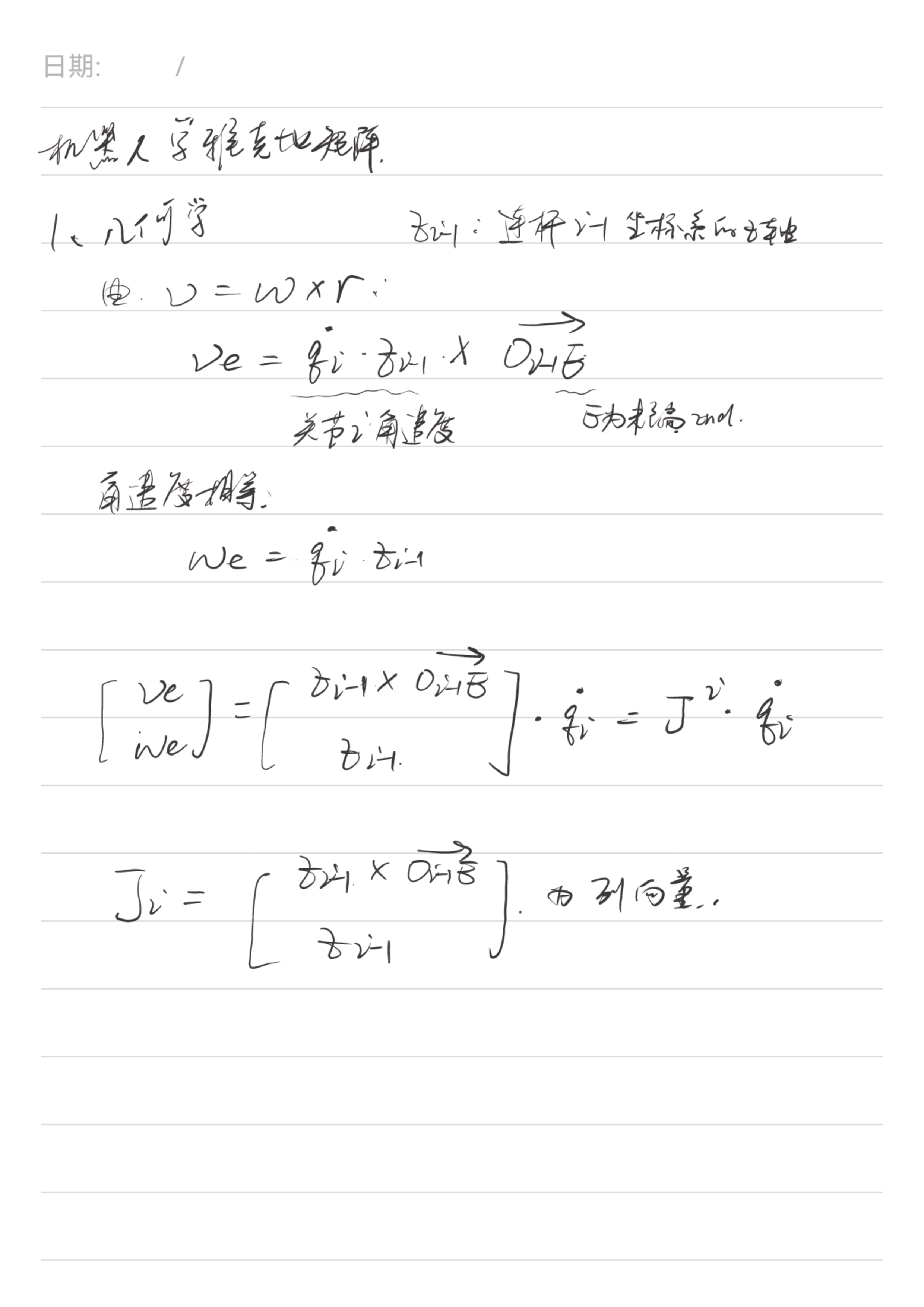
We call the Jacobian matrix obtained by describing the linear and angular velocities in Cartesian coordinates and the end effector’s velocity in the base frame of the manipulator as the reference system the basic Jacobian matrix; all other representations (e.g., changing Cartesian coordinates to cylindrical coordinates, spherical coordinates, changing angles to Euler angles or quaternion quaternions, etc.) can be converted from this basic Jacobian matrix. According to the definition of the basic Jacobian matrix above, the speed of the end effector can be written as follows:
\[\dot{x}=\left[\begin{array}{c} v_x \\ v_y \\ v_z \\ \omega_x \\ \omega_y \\ \omega_z \end{array}\right]=\left[\begin{array}{c} \vec{v} \\ \vec{\omega} \end{array}\right]\]Correspondingly, the Jacobian matrix can be written as:
\[J=\left[\begin{array}{l} J_v \\ J_\omega \end{array}\right]\]The upper part corresponds to the linear velocity and the lower part to the angular velocity.
Linear velocity component (Jv)
If our manipulator is a bit more complex and we need to use chi-square coordinate transformations to find the forwardkinematics formula, how should the Jacobian matrix be solved?
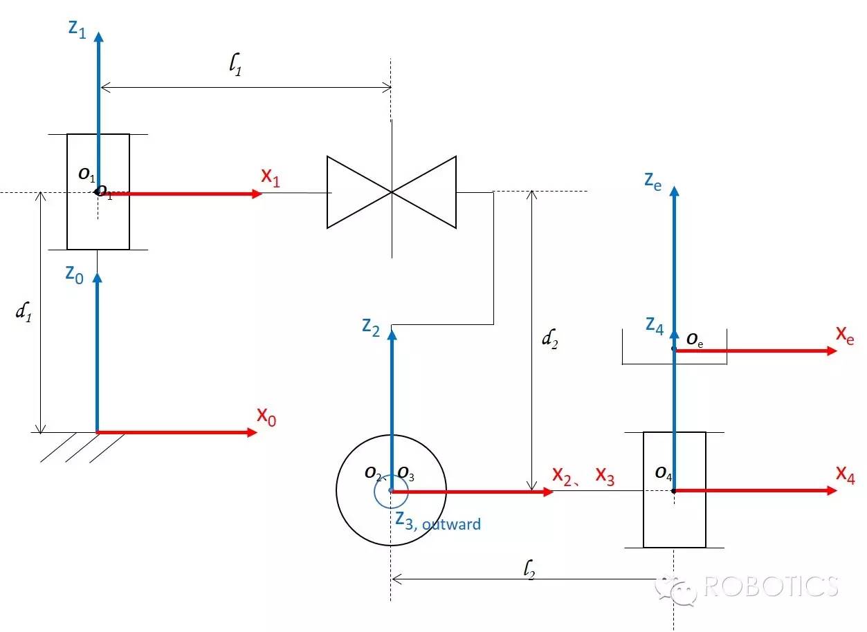
This is the forwardkinematics expression we derived for the end effector:
\[{ }_e^0 T=\left[\begin{array}{cccc} \times & \times & \times & l_2 c \theta_1 c \theta_3+l_1 c \theta_1 \\ \times & \times & \times & l_2 s \theta_1 c \theta_3+l_1 s \theta_1 \\ \times & \times & \times & l_2 s \theta_3+d_2 \\ 0 & 0 & 0 & 1 \end{array}\right]\]The only thing we need is the part of the figure circled by the red box, and if you are good at coordinate transformations, you should immediately see that it represents the position of the end effector w.r.t frame{0}. So, for Jv, we just need to take this 3×1 vector (xe, ye, ze) circled in the red frame and solve for the joint space vectors (θ1, d2, θ3, θ4)! Following the rules for vector derivation, we will get a 3×4 matrix as follows:
\[J_v=\left[\begin{array}{cccc} -l_2 s \theta_1 c \theta_3-l_1 s \theta_1 & 0 & -l_2 c \theta_1 s \theta_3 & 0 \\ l_2 c \theta_1 c \theta_3+l_1 c \theta_1 & 0 & -l_2 s \theta_1 s \theta_3 & 0 \\ 0 & 1 & l_2 c \theta_3 & 0 \end{array}\right]\]Angular velocity component (Jw)
Let’s start by looking at the simplest planar manipulator:
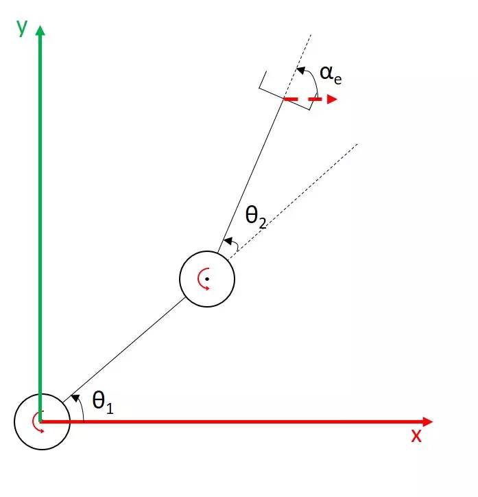
Of course, this time we are only concerned with the orientation of the end effector. For a planar manipulator, the end effector has only one degree of rotational freedom α, which is labelled in the figure (set to 0° when coinciding with the x-axis, and turning from the x-axis to the y-axis is a forwarddirection). At this point, our operation space is (α), and the joint space is still (θ1,θ2); by definition, we require the angular velocity part of the Jacobian matrix as follows:
\[J_\omega=\left[\begin{array}{ll} \frac{d \alpha}{d \theta_1} & \frac{d \alpha}{d \theta_2} \end{array}\right]\]For this planar manipulator, it is easy to see that: α will turn by as many angles as θ1 turns; ditto for θ2 - so Jw should be [1, 1]. What’s the point of this example? Hopefully it helps you to establish an intuitive impression and basic idea - how many angles a rotary joint of a manipulator turns around a certain axis, and how many angles its end effector turns around that axis accordingly; in the case of a planar manipulator, this means that the rotational speed of a rotary joint is multiplied by 1 to get the end effector that it causes ( Contribute) the speed of rotation of the end effector, so Jw above is [1, 1].
In three dimensions, angular velocity is defined as a vector pointing to an axis of rotation whose direction can be determined by the right-hand rule.Since we define each rotary joint of a manipulator as rotating about its own z-axis, when the rotational speed of a rotary joint is ω, the angular velocity vector of the end effector it contributes is necessarily [0, 0, ω] using the coordinate system of this rotary joint itself as the frame of reference. In other words, the rotational speed of this rotary joint multiplied by [0, 0, 1] yields the angular velocity of the end effector it contributes to (w.r.t the coordinate system of this rotary joint). (The actual rotational speed of the end effector can be linearly superimposed by the angular velocities of the different rotational joints contributing to it.)
Since our basic Jacobian matrix is in frame{0} as the reference system, in order to write Jw, we need to convert the z-axis [0, 0, 1] of each rotational joint, from being represented in the joint’s own coordinate system as the reference system, to the base coordinate system frame{0}. In addition, for the translational joints, since the motion of the translational joints cannot change the orientation of the end effector, the derivation of the orientation of the end effector to the position of the translational joints must be zero!
As an example, the RPRR manipulator that appeared earlier has a Jacobian matrix angular velocity part that looks like this:
\[J_\omega=\left[\begin{array}{llll} { }^0 \hat{z}_1 & \overrightarrow{0} & { }^0 \hat{z}_3 & { }^0 \hat{z}_4 \end{array}\right]\]Now the last question we have left is how to find the z-axis coordinates w.r.t frame{0} of each joint - in fact, after calculating the Homogeneous Transformation Matrices of each joint once, didn’t we already know the answer? Write out two of them for you:
\[{ }_1^0 T=\left[\begin{array}{cccc} \times & \times & 0 & \times \\ \times & \times & 0 & \times \\ \times & \times & 1 & \times \\ 0 & 0 & 0 & 1 \end{array}\right]{ }_3^0 T=\left[\begin{array}{ccccc} \times & \times & s \theta_1 & \times \\ \times & \times & -c \theta_1 & \times \\ \times & \times & 0 & \times \\ 0 & 0 & 0 & 1 \end{array}\right]\]The three elements of the third column are the $\hat{z}_1$ and $\hat{z}_3$.
Conclusion
- The upper part Jv of the fundamental Jacobian matrix is obtained by taking the derivative of the position vector of the end effector with respect to the joints;
-
The position vector of the end effector can be obtained from the forwardkinematics solution
-
the lower half of the fundamental Jacobian matrix Jw can be obtained from the unit vectors of the z-axis of each rotational joint written in the reference system of the base coordinate system
- Combining Jv and Jw gives an m×n matrix, where m is the degree of freedom of the end effector/operating space (for spatial manipulators usually m=6) and n is the number of joints in the manipulator.
Force Relationship
Having examined the position mapping relationship and velocity mapping relationship between joint space and operation space, we now ask another question: what about their force/torque mapping relationship?
The Jacobian matrix is likewise the link between the force/torque mapping relationship between joint space and operation space.
Now we are located in joint space and the force/torque output from the joint is:
\[\tau=\left[\begin{array}{llll} \tau_1 & \tau_2 & \ldots & \tau_n \end{array}\right]^T\]The speed of joint movement is:
\[\dot{q}=\left[\begin{array}{llll} \dot{q}_1 & \dot{q}_2 & \ldots & \dot{q}_n \end{array}\right]^T\]Then the power output of the whole system (equal to force times velocity) is expressed in joint space as
\[P=\tau^T \dot{q}\]Note that this is a vector dot product and P is a scalar.
Now from the point of view of the operating space, let the force/torque that the end effector is able to output to the outside world at this time (or the force/torque that the outside world exerts on the end effector in order to maintain the static equilibrium of the whole system) be:
\[F=\left[\begin{array}{llllll} f_1 & f_2 & f_3 & n_1 & n_2 & n_3 \end{array}\right]^T\]where f denotes the force and n denotes the torque. The velocity of the end effector is then
\[\dot{x}=\left[\begin{array}{llll} \dot{x}_1 & \dot{x}_2 & \ldots & \dot{x}_n \end{array}\right]^T\]Then the power of the external force applied to the end effector to do work on the whole system is
\[P=F^T \dot{x}\]By the law of conservation of energy, we must have
\[P=\tau^T \dot{q}=F^T \dot{x}\]Substitute the equation for instantaneous kinematics:
\[\begin{gathered} \tau^T \dot{q}=F^T J \dot{q} \\ \tau^T=F^T J=\left(J^T F\right)^T \\ \tau=J^T F \end{gathered}\]After a long derivation, we get another important use of the Jacobian matrix: the transpose of J multiplied by the force/torque in the operation space gives the force/torque output in the joint space! This is a mapping from the operation space to the joint space, in the opposite direction of the positive kinematics and instantaneous kinematics we talked about before.
So what is the point of learning this force mapping relationship for a real manipulator? For the most traditional position-controlled robots, which rely on sensing the position accurately, this equation may indeed be of little use. However, more and more applications require robots to be able to maintain a specific force at a certain position/direction (e.g., gripping an object, cleaning a glass), or to work safely in a complex environment (to ensure that it does not exert too much force on an object when it hits an obstacle); this mapping is essential to achieve such control.
Singularity
Simply put, Singularity is the loss of directional freedom of the end effector when the manipulator is in a certain configuration (i.e., a particular combination of joint positions) - the moment your manipulator is straight, your hand will never be able to move in the direction of your manipulator.
Now with the Jacobi Matrix, we can re-conceptualise Singularity from a mathematical point of view. Don’t forget the use of the Jacobian matrix: the velocity of the joints is multiplied by the Jacobian matrix to get the velocity of the end effector. The end effector loses degrees of freedom in a certain direction, which means that at the moment the manipulator reaches that configuration, the velocity of the end effector in that direction will always be 0, no matter how the joints move.
From a linear algebra point of view, the J-matrix at this point has the property that for all arbitrary vectors a, the multiplication of Ja yields a vector b. The dimension of the linear space consisting of all the vectors b will be at least one degree of freedom less than in the normal case - this indicates that the Jacobian matrix at this point in time has been down-ranked.
where the Jacobian matrix is:
\[J=\left[\begin{array}{ll} \frac{d x_e}{d \theta_1} & \frac{d x_e}{d \theta_2} \\ \frac{d y_e}{d \theta_1} & \frac{d y_e}{d \theta_2} \end{array}\right]=\left[\begin{array}{cc} -\sin \left(\theta_1+\theta_2\right)-\sin \theta_1 & -\sin \left(\theta_1+\theta_2\right) \\ \cos \left(\theta_1+\theta_2\right)+\cos \theta_1 & \cos \left(\theta_1+\theta_2\right) \end{array}\right]\]Now, in order to find at what configuration the manipulator encounters a singularity, i.e., to find when this Jacobian matrix is not a full rank matrix, we can directly use the fact that at this point the eigenvalue of J is 0 (i.e., at this point J is a singularity matrix) to find it:
\[\operatorname{det}(J)=-\cos \left(\theta_1+\theta_2\right)\left(\sin \left(\theta_1+\theta_2\right)+\sin \theta_1\right)+\sin \left(\theta_1+\theta_2\right)\left(\cos \left(\theta_1+\theta_2\right)+\cos \theta_1\right)=0\]so as to
\[\begin{gathered} \sin \left(\theta_1+\theta_2\right) \cos \theta_1-\cos \left(\theta_1+\theta_2\right) \sin \theta_1=0 \\ \sin \left(\theta_1+\theta_2-\theta_1\right)=\sin \theta_2=0 \end{gathered}\]So the singular configuration is θ2 = 0. At this point, the manipulator is “straight” and the end effector cannot move in the direction of the manipulator link. Substituting this value into the original matrix reveals that the row/column vectors of J are not linearly independent, and have rank 1.
Mathematically, the statement of singular matrices is only valid for square matrices, and finding eigenvalues is also only valid for square matrices. For robots, (Kinematic) Singularity is a downscaling of the robot’s end effector motion space at a certain configuration, and has nothing to do with the shape of the Jacobian matrix - it’s just that when the Jacobian matrix isn’t a square matrix, we need to get rid of the redundant degrees of freedom away before solving.
Redundancy
Speaking of redundant degrees of freedom, I’m sure you can already figure out how to see redundancy from the Jacobian matrix - when it’s short and fat that is. Your hand was also used as an example in the first post, because the human hand has seven degrees of freedom in joint space, so you are able to move your elbow with your hand fixed. Mathematically, this means
\[\exists \dot{q}, J \dot{q}=0\]We know that if A is a square matrix, then a sufficient condition for Ax=0 to have non-zero solutions is that A is a singular matrix - that is, if there are no redundant degrees of freedom, the case of a manipulator whose joints move and whose end effector doesn’t move can only occur when it is in singularity. However, if A is a fat matrix, then Ax=0 must have an infinite number of non-zero solutions, and the space of these solutions is called the null space.
To mention briefly: for a robot with redundant degrees of freedom, suppose you want to control the end effector to move to a certain position, but also make sure that its elbow does not hit an obstacle during the process, then you can always find a set of solutions in nullspace to meet your requirements: avoid obstacles without changing the trajectory of the end effector. Such a method is called null space control.