Cable Driven Manipulator 1 - Structural Design
Based on the overall needs and design performance index requirements of the cable-driven manipulator, the joints are assigned as shoulder, elbow and wrist. The shoulder and wrist joints include 3-DOF in pitch, yaw, and rotation, and the elbow joint is responsible for 1-DOF in pitch, and the shoulder, elbow, and wrist joints are connected with each other to form the overall arm.
7-DOF Manipulator

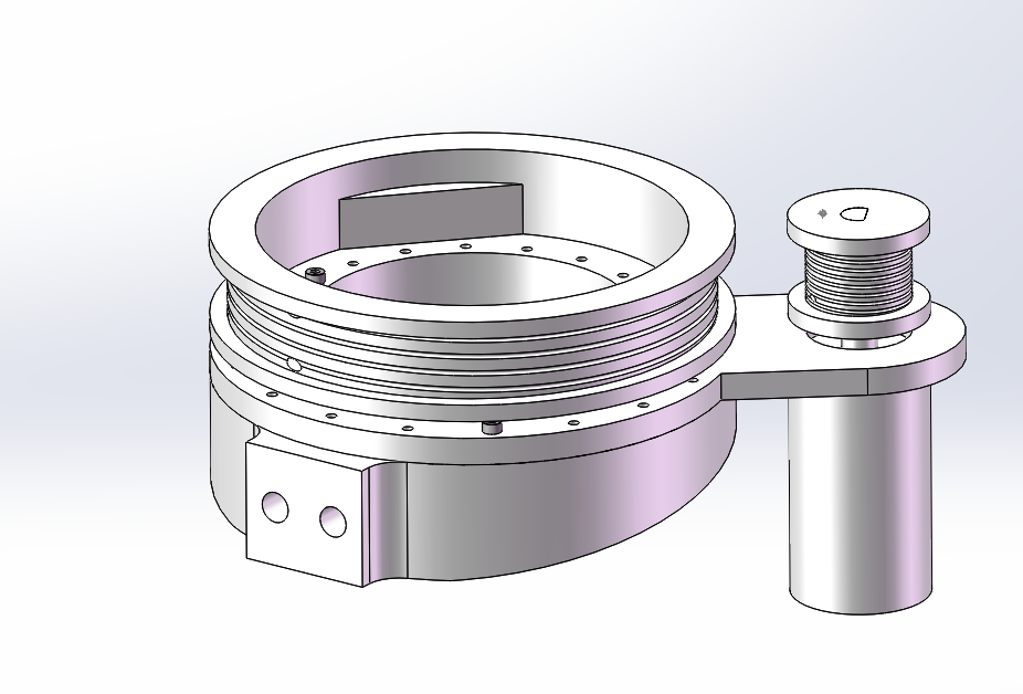
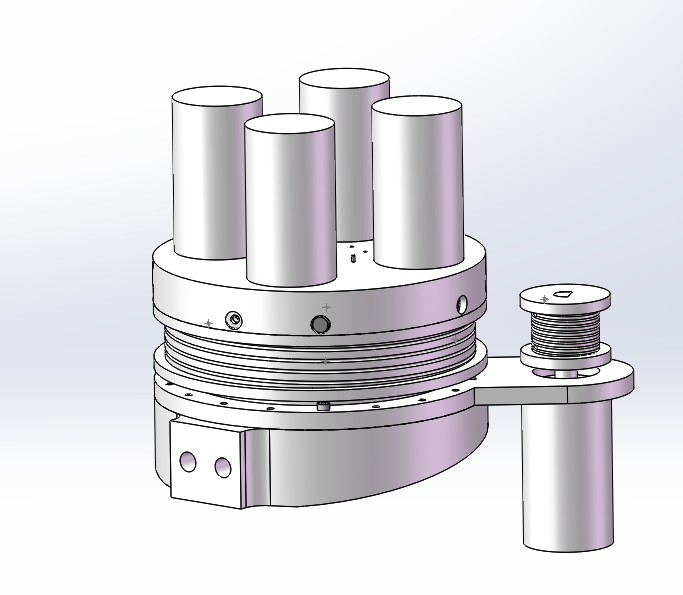
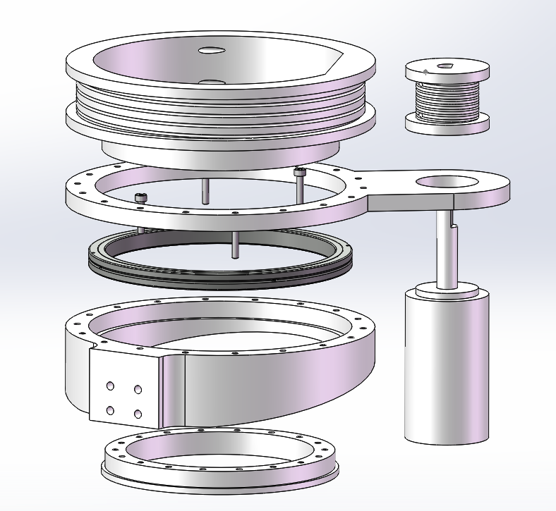
Shoulder Mechanism
Paper
[1] Anthropomorphic Low-Inertia High-Stiffness Manipulator for High-Speed Safe Interaction
[2] 绳驱七自由度仿人机械臂设计及其运动控制方法研究
[3] Development of Low-Inertia High-Stiffness Manipulator LIMS2 for High-Speed Manipulation of Foldable Objects
Concept
-
3 joints in series for 3-DoF
-
capstan drive mechanisms
Detail
V1.0
V2.0
Elbow Mechanism
Paper
[1] Anthropomorphic Low-Inertia High-Stiffness Manipulator for High-Speed Safe Interaction
[2] 绳驱七自由度仿人机械臂设计及其运动控制方法研究
[3] 一类绳驱机械臂的控制系统设计与实现
Concept
refer to Wrist Mechanism
Detail
V1.0
V2.0
V2.1
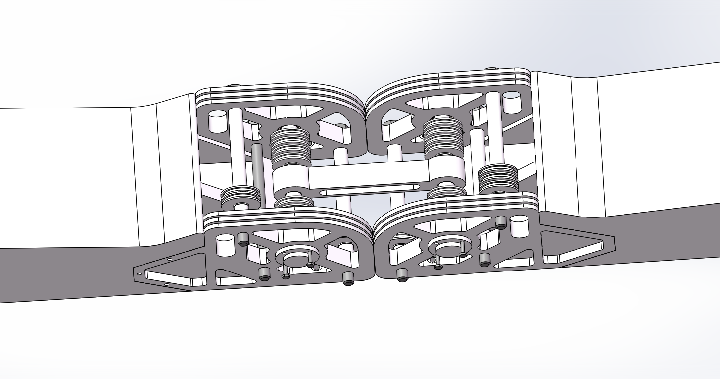
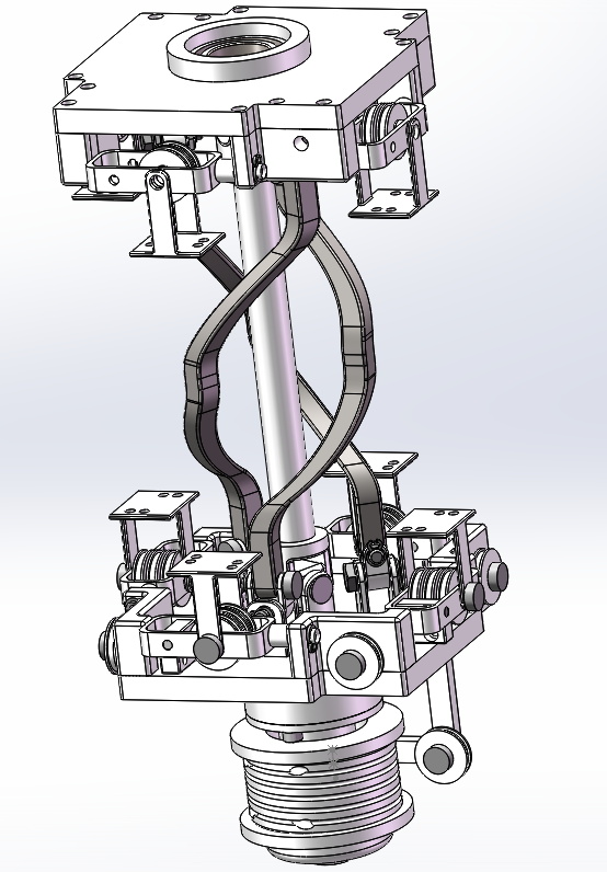
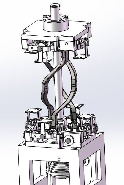
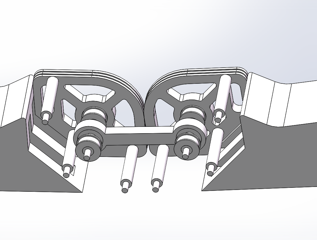
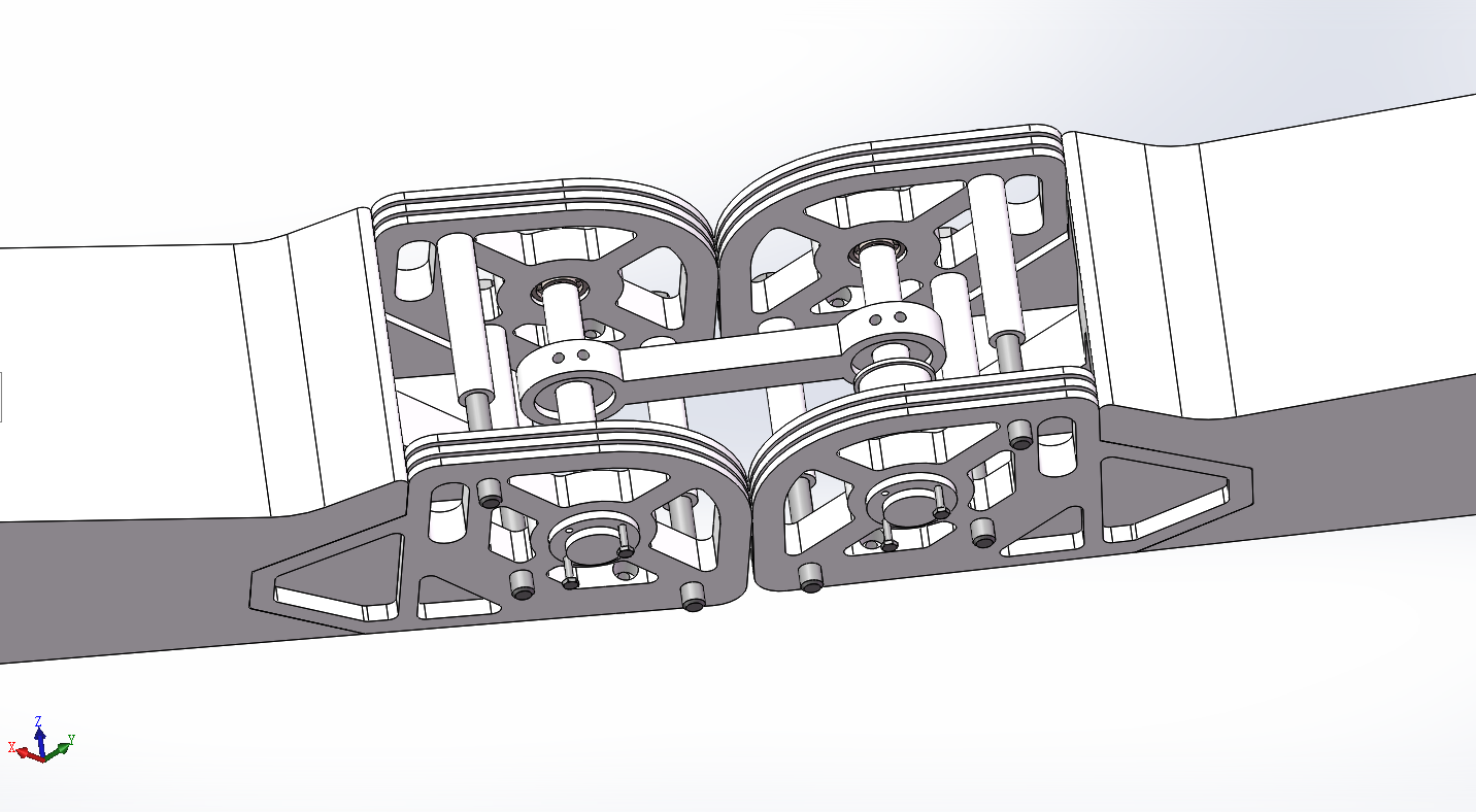
Wrist Mechanism
Paper
[1]Quaternion Joint: Dexterous 3-DOF Joint Representing Quaternion Motion for High-Speed Safe Interaction
Abstract
-
It has a 2-DOF spherical pure rolling joint and a 1-DOF rotation joint at the distal end;
-
To precisely approximate the spherical pure rolling motion, a novel parallel mechanism composed of three identical supporting linkages.
Concept
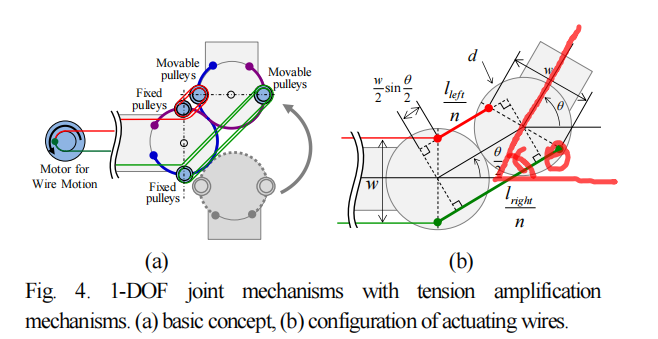
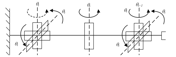
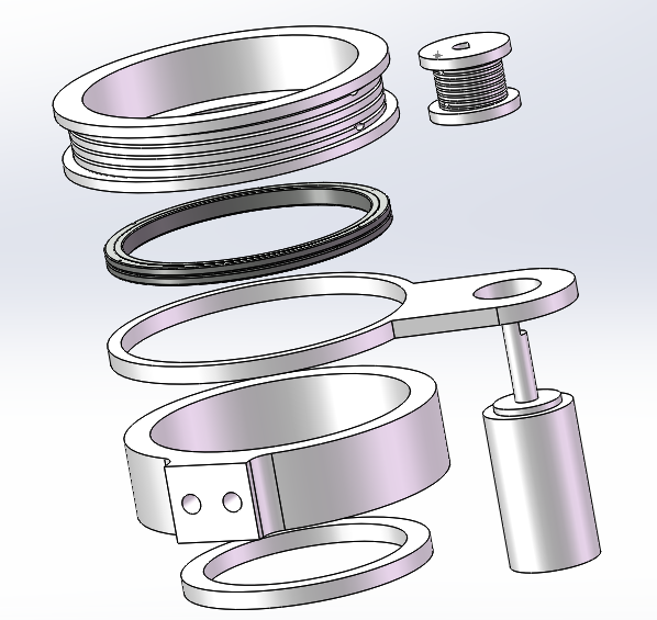
The two coupling wires are connected along the circular rolling surface (the blue and purple wires in the figure), enabling a pure rolling motion without slippage. The actuating wires (red and green wires) are placed around the freely rotating fixed and movable pulley sets multiple times, which amplifies the wire tension.
The displacements of the left and right wires, 𝑙𝑙𝑒𝑓𝑡 and 𝑙𝑟𝑖𝑔ℎ𝑡 , have the same magnitude but opposite direction, as indicated in the following:
\[l_{\text {left }}=-l_{\text {right }}=n w \sin \frac{\theta}{2} \text {}\]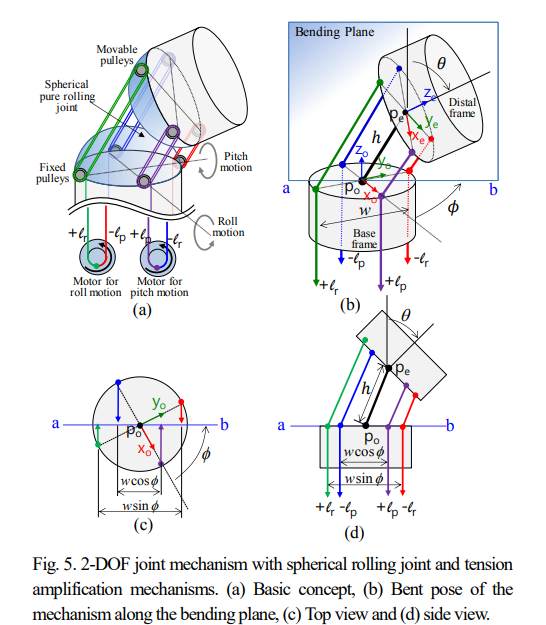
There are two hemispherical rolling surfaces instead of circular-shaped parts, which are surrounded by four actuation wires for the 2-DOF bending motion.
This joint also can be actuated using two motors. Consider a bending plane, where the two centerlines of the base frame and distal frame coexist.
\[\begin{aligned} & l_r=l_r^{+}=-l_r^{-}=n w \sin \phi \sin \frac{\theta}{2} \\ & l_p=l_p^{+}=-l_p^{-}=n w \cos \phi \sin \frac{\theta}{2} \end{aligned}\]An anti-parallelogram mechanism can produce a pure rolling motion along two ellipses.
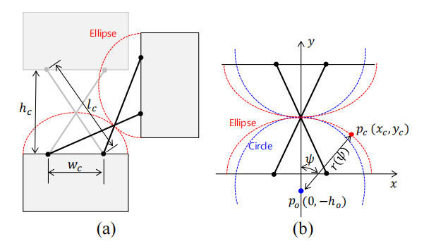
The ellipse equation is as follows:
\[\frac{x_c{ }^2}{\left(l_c / 2\right)^2}+\frac{y_c{ }^2}{\left(h_c / 2\right)^2}=1\]Assume that there is a circle that properly approximates this ellipse, and that its center 𝑝𝑜 is placed along the y-axis with offset ho
Considering a line from 𝑝𝑜 to a point on the ellipse 𝑝𝑐 , the line equation and length of the line 𝑟 are respectively:
\[\begin{aligned} y_c & =\frac{1}{\tan \psi} x_c-h_o \\ r & =x_c / \sin \psi \end{aligned}\]By solving 𝑥c the length 𝑟 can be represented as a function of 𝜓 as follows:
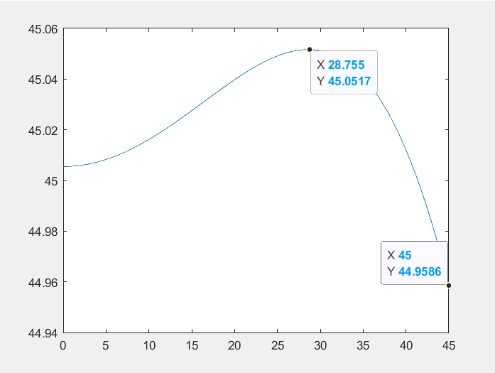
\[r(\psi)=\frac{h_o+\sqrt{\left.h_o{ }^2+\left(1+\left(\frac{w_c}{h_c}\right)^2 \tan ^2 \psi\right)\right)\left(\left(\frac{w_c}{2}\right)^2-h_o{ }^2\right)}}{\left.\cos \psi\left(1+\left(\frac{w_c}{h_c}\right)^2 \tan ^2 \psi\right)\right)}\]Set ho, wc and hc, if the 𝑟 remains a near constant, it can be considered that it can approximate the rolling motion between two circles.
wc = 30; lc = 85.75; ho = 4.84, Calculations using matlab:
wc = 30;
lc = 85.75;
ho = 4.84;
hc = (lc * lc - wc * wc) ^ 0.5;

N = 1000;
phi = zeros(1,N);
r = zeros(1,N);
numerator = zeros(1,N);
denominator = zeros(1,N);
value1 = zeros(1,N);
value2 = zeros(1,N);
value3 = zeros(1,N);

for k = 1:N
     phi(k) = k * 45 / N;
%     value1 = ho * ho;
%     value2 = 1 + wc * wc / hc / hc * tan(phi(k)) * tan(phi(k));
%     value3 = wc * wc / 4 - ho * ho;
%     numerator = (value1 + value2 * value3)^0.5 + ho;
% %     numerator = ho + (ho * ho + (1 + wc * wc / hc / hc * tan(phi(k)) * tan(phi(k))) * (wc * wc / 4 - ho * ho))^0.5;
%     denominator = cos(phi(k)) * (1 + wc * wc / hc / hc * tan(phi(k)) * tan(phi(k)));

    value1(k) = hc^4/4/lc/lc*tan(deg2rad(phi(k)))^2;
    value2(k) = hc^2/4;
    value3(k) = hc^2*ho^2/lc/lc*tan(deg2rad(phi(k)))^2;
    numerator(k) = (value1(k) + value2(k) - value3(k))^0.5 + ho;
    denominator(k) = cos(deg2rad(phi(k))) * (1 + hc^2/lc/lc * tan(deg2rad(phi(k)))^2);

    r(k) = numerator(k) / denominator(k);
end

figure();
plot(phi,r)
Detail
V1.0
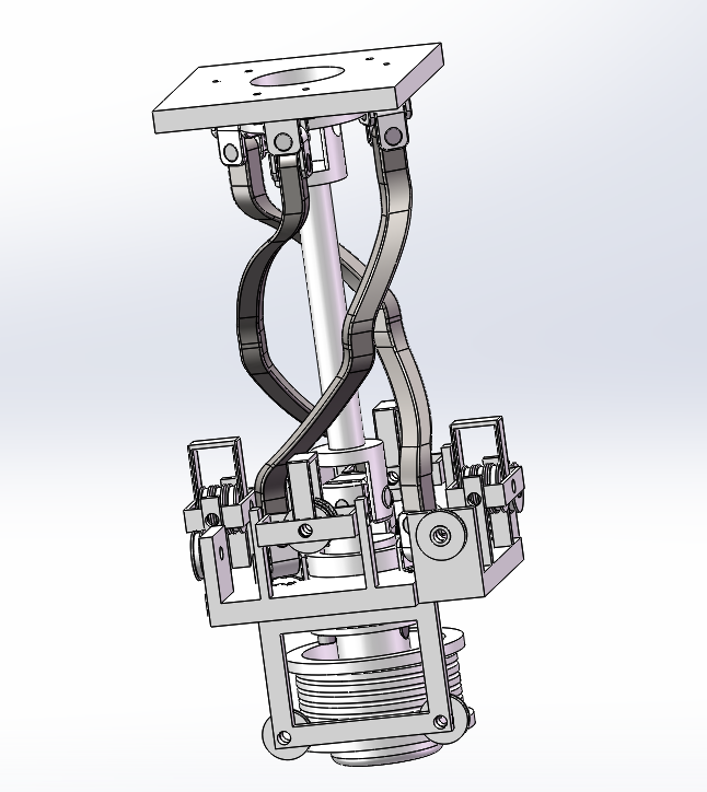
V2.0
wc = 30; lc = 85; ho = 5;